library(tidyverse)Data Transformation
Session 2b
“Transformation includes narrowing in on observations of interest (like all people in one city or all data from the last year), creating new variables that are functions of existing variables (like computing speed from distance and time), and calculating a set of summary statistics (like counts or means).”
–https://r4ds.hadley.nz/intro
In tidyverse framework, dplyr is the main package used for data transformation. The following goes through a list of popular functions that help you manipulate your data. Using the Twitter example data we imported last week, we will start with wrangling the columns (i.e., variables) and then switch to rows (i.e., observations.)
Let’s first load tidyverse and import the drob_tweets data that we’ve imported last week.
drob_tweets<-read_delim(file="https://raw.githubusercontent.com/dgrtwo/tidy-text-mining/master/data/tweets_dave.csv",
                        col_types = cols(tweet_id =col_character(),
                                         in_reply_to_status_id = col_character(),
                                         in_reply_to_user_id = col_character(),
                                         timestamp = col_datetime(format = "%Y-%m-%d %H:%M:%S %z"),
  source = col_character(),
  text = col_character(),
  retweeted_status_id = col_character(),
  retweeted_status_user_id = col_character(),
  retweeted_status_timestamp = col_datetime("%Y-%m-%d %H:%M:%S %z"),
expanded_urls = col_character()))glimpse(drob_tweets)Rows: 4,174
Columns: 10
$ tweet_id <chr> "816108564720812032", "815892641820901376",…
$ in_reply_to_status_id <chr> NA, NA, NA, NA, NA, "815320862660366336", N…
$ in_reply_to_user_id <chr> NA, NA, NA, NA, NA, "3230388598", NA, "1425…
$ timestamp <dttm> 2017-01-03 02:26:59, 2017-01-02 12:08:59, …
$ source <chr> "<a href=\"http://twitter.com/download/ipho…
$ text <chr> "RT @ParkerMolloy: 2017 is off to quite a s…
$ retweeted_status_id <chr> "816082588137881600", "776081137722650628",…
$ retweeted_status_user_id <chr> "634734888", "2842614819", "69133574", "756…
$ retweeted_status_timestamp <dttm> 2017-01-03 00:43:45, 2016-09-14 15:32:16, …
$ expanded_urls <chr> "https://twitter.com/ParkerMolloy/status/81…1 Manipulating columns
1.1 Create new columns

We use mutate() to create new variables that are functions of existing variables. The original dataset will not be altered.
Let’s create a few time related variables from the existing timestamp variable.
drob_tweets_1<- mutate(drob_tweets, # original data
                       year=year(timestamp), # new vars. = f(existing vars.)
                       month=month(timestamp),
                       month2=month(timestamp, label = T),
                       day=day(timestamp),
timestamp.ymd=as_date(timestamp))1.2 Select and remove columns
Now, I only want to examine the time variables so I use select() to keep these variables.
drob_tweets_YM<-select(drob_tweets_1,
                       c(timestamp, year, month, month2, day, timestamp.ymd))

glimpse(drob_tweets_YM)
Rows: 4,174
Columns: 6
$ timestamp <dttm> 2017-01-03 02:26:59, 2017-01-02 12:08:59, 2017-01-01 19…
$ year <dbl> 2017, 2017, 2017, 2017, 2017, 2016, 2016, 2016, 2016, 20…
$ month <dbl> 1, 1, 1, 1, 1, 12, 12, 12, 12, 12, 12, 12, 12, 12, 12, 1…
$ month2 <ord> 1月, 1月, 1月, 1月, 1月, 12月, 12月, 12月, 12月, 12月, 12月, 12月, 1…
$ day <int> 3, 2, 1, 1, 1, 31, 31, 30, 29, 29, 29, 29, 29, 29, 29, 2…
$ timestamp.ymd <date> 2017-01-03, 2017-01-02, 2017-01-01, 2017-01-01, 2017-01…Of course, we can also use select() to remove variables.
drob_tweets_lite<-select(drob_tweets_1,
                       -c(in_reply_to_user_id, # use minus to de-select
                          retweeted_status_id:expanded_urls)) #   use colon to specify a sequence of variables
glimpse(drob_tweets_lite)
Rows: 4,174
Columns: 10
$ tweet_id <chr> "816108564720812032", "815892641820901376", "815…
$ in_reply_to_status_id <chr> NA, NA, NA, NA, NA, "815320862660366336", NA, "8…
$ timestamp <dttm> 2017-01-03 02:26:59, 2017-01-02 12:08:59, 2017-…
$ source <chr> "<a href=\"http://twitter.com/download/iphone\" …
$ text <chr> "RT @ParkerMolloy: 2017 is off to quite a start.…
$ year <dbl> 2017, 2017, 2017, 2017, 2017, 2016, 2016, 2016, …
$ month <dbl> 1, 1, 1, 1, 1, 12, 12, 12, 12, 12, 12, 12, 12, 1…
$ month2 <ord> 1月, 1月, 1月, 1月, 1月, 12月, 12月, 12月, 12月, 12月, 12月…
$ day <int> 3, 2, 1, 1, 1, 31, 31, 30, 29, 29, 29, 29, 29, 2…
$ timestamp.ymd <date> 2017-01-03, 2017-01-02, 2017-01-01, 2017-01-01,…1.3 Rename columns
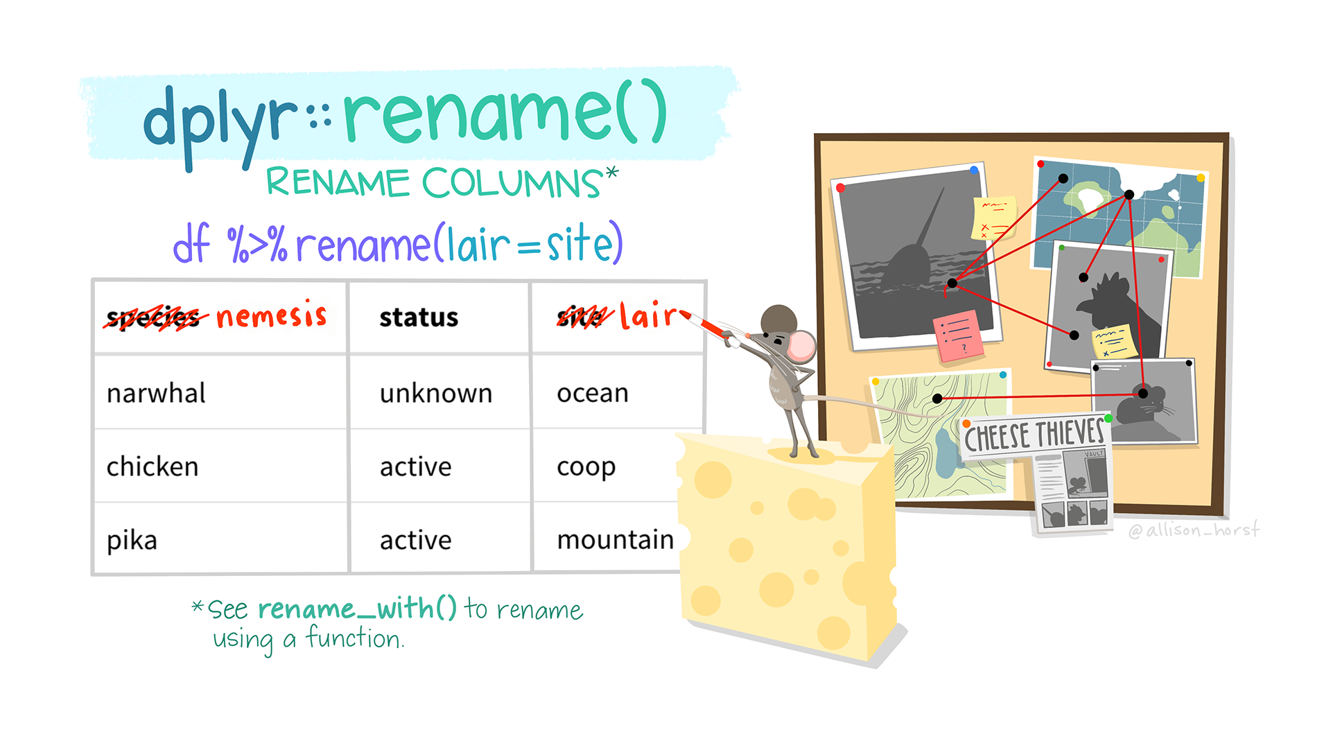
We use rename() to assign new names to existing variables. Here, I rename month2 to letter.month.
drob_tweets_2<-rename(drob_tweets_1,
                      letter.month=month2, # new name = old name
                      tweet=text)


colnames(drob_tweets_2)
[1] "tweet_id" "in_reply_to_status_id"
[3] "in_reply_to_user_id" "timestamp"
[5] "source" "tweet"
[7] "retweeted_status_id" "retweeted_status_user_id"
[9] "retweeted_status_timestamp" "expanded_urls"
[11] "year" "month"
[13] "letter.month" "day"
[15] "timestamp.ymd" 1.4 Relocate column positions

For a better view of the data set, I move the newly created time variables to be together with timestamp and right after tweet. In this task, we userelocate().
drob_tweets_3<- relocate(drob_tweets_2,
                         c(year, month, letter.month, day, timestamp, timestamp.ymd),
                         .after = tweet)

colnames(drob_tweets_3)
[1] "tweet_id" "in_reply_to_status_id"
[3] "in_reply_to_user_id" "source"
[5] "tweet" "year"
[7] "month" "letter.month"
[9] "day" "timestamp"
[11] "timestamp.ymd" "retweeted_status_id"
[13] "retweeted_status_user_id" "retweeted_status_timestamp"
[15] "expanded_urls" 2 Pipes
You might find something tedious here. We created many new but unnecessary data sets whenever we executed a new function. Also, if we want to perform multiple functions simultaneously, we must use many parentheses, making your script hard to read. See the following ridiculous codes.
drob_tweets_4<-relocate(rename(mutate(drob_tweets, # original data
                       year=year(timestamp), # new vars. = f(existing vars.)
                       month=month(timestamp),
                       month2=month(timestamp, label = T),
                       day=day(timestamp),
                       timestamp.ymd=as_date(timestamp)),

                       letter.month=month2, # rename vars.
                       tweet=text),

                       c(year, month, letter.month, timestamp), # relocating vars.
                         .after = tweet)
Luckily, this issue can be easily solved by using a pipe operator %>% from the magrittr package of the tidyverse family. You may read it as “and then,” which pipes an object forward to a function or call expression. Let’s see how we can use it by only creating one new date set while executing all the above functions.
drob_tweets.df<-drob_tweets %>%
  mutate(year=year(timestamp), # new vars. = f(existing vars.)
         month=month(timestamp),
         month2=month(timestamp, label = T),
         day=day(timestamp),
         timestamp.ymd=as_date(timestamp)) %>%
  rename(letter.month=month2, # rename vars.
         tweet=text) %>%
  relocate(c(year, month, letter.month, day, timestamp,timestamp.ymd), # relocate vars.
           .after = tweet) %>%
  select(-c(in_reply_to_user_id,
retweeted_status_id:expanded_urls)) glimpse(drob_tweets.df)Rows: 4,174
Columns: 10
$ tweet_id <chr> "816108564720812032", "815892641820901376", "815…
$ in_reply_to_status_id <chr> NA, NA, NA, NA, NA, "815320862660366336", NA, "8…
$ source <chr> "<a href=\"http://twitter.com/download/iphone\" …
$ tweet <chr> "RT @ParkerMolloy: 2017 is off to quite a start.…
$ year <dbl> 2017, 2017, 2017, 2017, 2017, 2016, 2016, 2016, …
$ month <dbl> 1, 1, 1, 1, 1, 12, 12, 12, 12, 12, 12, 12, 12, 1…
$ letter.month <ord> 1月, 1月, 1月, 1月, 1月, 12月, 12月, 12月, 12月, 12月, 12月…
$ day <int> 3, 2, 1, 1, 1, 31, 31, 30, 29, 29, 29, 29, 29, 2…
$ timestamp <dttm> 2017-01-03 02:26:59, 2017-01-02 12:08:59, 2017-…
$ timestamp.ymd <date> 2017-01-03, 2017-01-02, 2017-01-01, 2017-01-01,…Now, we can remove the other date sets created earlier.
rm(list = ls(pattern="drob_tweets_"))See how %>% can help improve your coding efficiency and script readability. You may also see |> somewhere else, a native pipe operator added to base R since the recent R 4.1.0 version. %>% and |> work similarly while with some differences. You may read more on this here. There are other pip operators from magrittr. We will see one more example later very soon.
3 Working on rows
Here, we start with filtering tweets that are 1) from 2012 to 2015 and 2) are not retweets. The function filter() subsets a data frame satisfying the specified conditions.
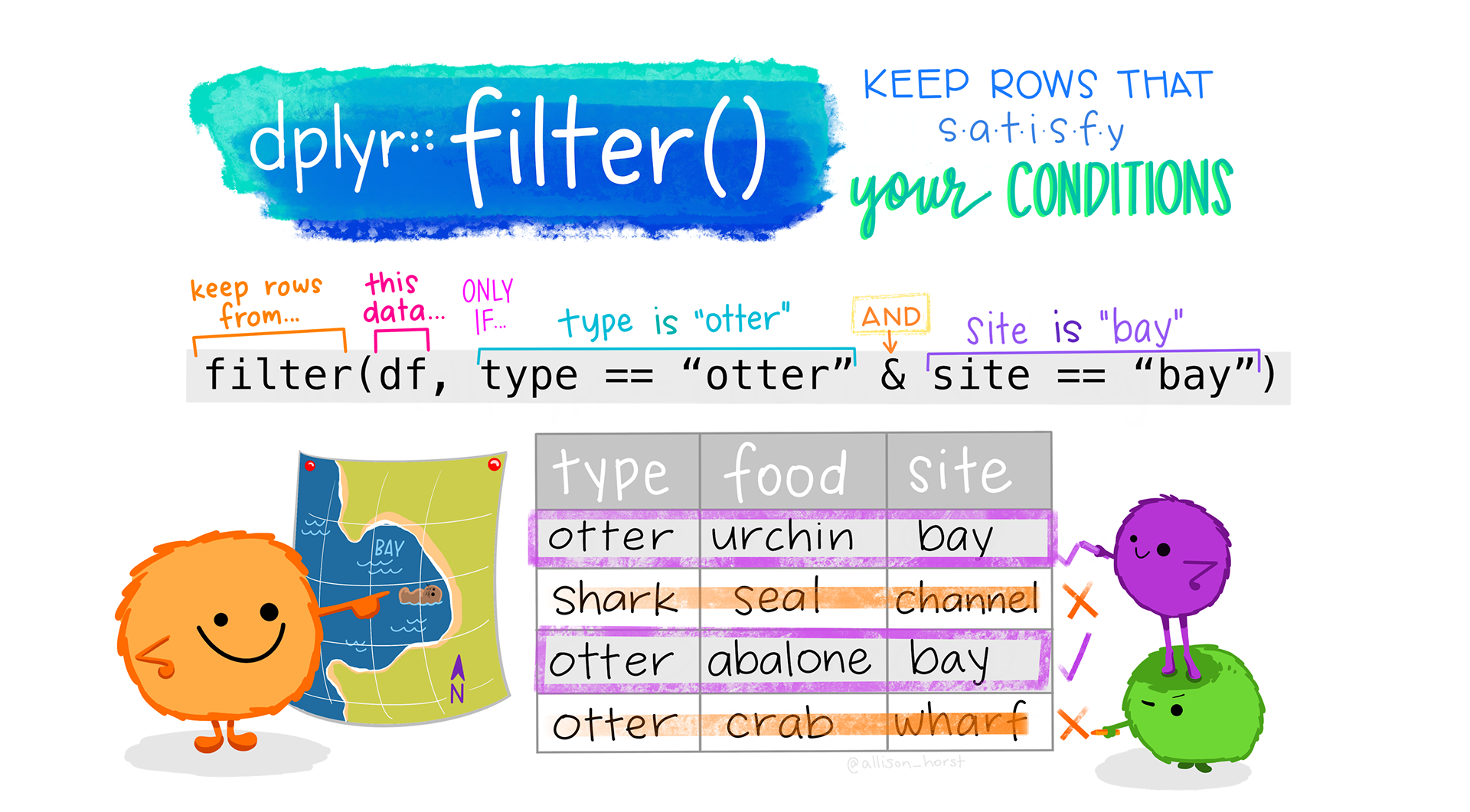
We then arrange the tweet from the newest year to the oldest while keeping the year and day in ascending order using the arrange() function.
drob_tweets.df2 <-drob_tweets.df %>%
  filter(year>=2012 & year<=2015) %>% # keep tweets from 2012-2015
  filter(!is.na(in_reply_to_status_id)) %>% # keep the reply tweets (defined soly based on this variable)
arrange(desc(year), month, day) # re-order the tweets sequence by timeView(drob_tweets.df2)
4 Many more useful functions…
dplyr has many more useful functions to conduct a variety of tasks. In the following example, I further show a few commonly used functions, particular those ones are useful in manipulating data by groups and computing aggregated statistics.
Example: Retweeting events
We might want to examine users’ retweeting behavior (as it might be a factor contributing to the users’ follower/following network size.)
To know a user’s activeness of retweeting, we may calculate how many retweets per month in each year.
drob_tweets.YMgroup<-drob_tweets.df2 %>%
  group_by(year, month) %>%
  mutate(reply.tweet.count.YM=n(),
         reply.daysYM=n_distinct(timestamp.ymd)) %>%
  ungroup() %>% # always ungroup when a grouping task is finished
  group_by(year) %>%
  mutate(reply.monthsY=n_distinct(month)) %>%
  ungroup() %>%
  select(year, month, timestamp.ymd,
         reply.tweet.count.YM,reply.daysYM,reply.monthsY)

View(drob_tweets.YMgroup)
Now we can tell how many months that this user has active retweeting events each year.
drob_tweets.YMgroup %>%
  distinct(reply.monthsY, year)
# A tibble: 4 × 2
reply.monthsY year
<int> <dbl>
1 12 2015
2 5 2014
3 4 2013
4 2 2012Further, we can show the most active retweeting months each year. Let’s take a look at the most active top 3 months.
drob_tweets.YMtop3<-drob_tweets.YMgroup %>%
  distinct(year, month, .keep_all=T) %>% # keep distinct rows at year-month level and keep all variables.
  group_by(year)%>%
  slice_max(order_by=reply.tweet.count.YM, # sort by number of retweets
            n=3, # specify that we only want the top 3
            with_ties=T) %>%  # keep the rows of ties
  ungroup()%>%
select(-timestamp.ymd) # as we are computing aggregated statistics at the year and month levels, we disregard the day level variable for clarity. View(drob_tweets.YMtop3)
What can we tell from the above tables?
You can see that there are only two lines of data entry for 2012. That’s because the user only retweeted in two months (i.e., Jan. and Jun.) in 2012. See the corresponding reply.monthsY value is 2.
In 2013, four months shown up since we specified that we want to include the ties. Thus, the four months have retweets and each has only one retweet are all “sliced”.
In 2014, the user has a little bit more engagement in retweeting during five months. Notably, December had the highest number of replied tweets, with September and February following closely.
At last, the number of retweets significantly increased in 2015. I wonder what happened this year. Also, Dec. is an active retweeting month. Now, take a wild guess: in which year did this user have a larger tweeting network?
Finally, we can use summarize() to compute active retweeting statistics at the day level.
drob_tweets.group<-drob_tweets.df2 %>%
  group_by(timestamp.ymd) %>%
  summarise(reply.tweet.daily=n()) %>%
  ungroup() %>%
  mutate(mean.reply.tweet.daily=mean(reply.tweet.daily),
         sd.reply.tweet.daily=sd(reply.tweet.daily),
         reply.days=n_distinct(timestamp.ymd)) %>%
arrange(desc(reply.tweet.daily))drob_tweets.group2<-drob_tweets.df2 %>%
mutate(reply.days=n_distinct(timestamp.ymd)) %>%
group_by(timestamp.ymd) %>%
summarise(reply.tweet.count.daily=n()) %>%
ungroup() 5 Other tools for cleaning dirty data
In addition to dplyr and lubridate that we have explored so far for data cleaning and manipulation, janitor is another handy tool to deal with dirty data. Take a look of its vignettes, see how it can help with cleaning column names, removing rows and columns, exploring duplication patterns, cleaning datetime data, and so much more.
6 Dealing with BIG data
So far, we have used two example datasets to demonstrate data importing and wrangling. These two datasets are small in terms of size and are snapshots of penguins and tweets. We worked with these data in data frames, which are processed through our computer’s Random Access Memory (RAM).
As you progress in your CSS journey, we would encounter with large datasets that exceeding the RAM limit. In such instances, managing big data is better handled through databases and database management systems (DBMS). The resources provided below offer introductory strategies for utilizing R in dealing with big data. However, comprehensive training on handling big data goes beyond the scope of this class.
Importing big data from database using
DBIanddbplyr.Officially recommended strategies for working with big data in R.
7 Reflection: working with GenAI
As we wrap up this session, take a moment to reflect on your experience using GenAI as a learning tool while working through the activities. GenAI can be powerful aids when used thoughtfully, but they are most effective when paired with your critical thinking and coding practice.
Take 5–10 minutes to jot down your thoughts on your experience so far. Here are some example questions to guide your reflection:
1) Did GenAI help you understand any concepts more clearly (e.g., debugging, understanding mutate() or group_by())?
2) Were there moments where you felt relying on GenAI might have hindered your learning? How did you address this? Relevently, how did you balance using GenAI with your own problem-solving skills?
3) Did you notice any inaccuracies or limitations in the responses provided by GenAI? How did you verify the information it gave you?
4) What strategies will you use in future sessions to make your interactions with GenAI more effective and aligned with your learning goals?