#install.packages(c("tidytext", "sotu", "ggwordcloud", "quanteda",  "textstem"))

library(tidytext) # Text preparation and analysis package in tidyverse framework
library(sotu) # Data

library(ggwordcloud) # A ggplot2 extension fo drawing word clouds
library(quanteda) # Another text preparation and analysis package
library(textstem) #Implements stemming and lemmatization
library(tidyverse) Tokenization and Preprocessing
Session 3a
1 Recap: Workflow of text analysis
In a basic text analysis, we start with acquiring text data (i.e., selection) and representing the content quantitatively (i.e.,representation). We then extract the textual features and move to quantitative or computational analysis.
In our four R sessions for the Text-as-data module, we will practice this workflow mainly using an R package called tidytext, which is designed to work seamlessly within the tidyverse ecosystem packages, such as dplyr and ggplot2. It also integrates well with other text analysis R packages, such as quanteda and tm, allowing users to combine text-as-data techniques with statistical analysis, data visualization, and machine learning methods, all within a unified and coherent workflow.
You can find (almost) all text-as-data related R packages in this awesome list: CRAN Task View: Natural Language Processing (r-project.org)
1.1 Agenda today
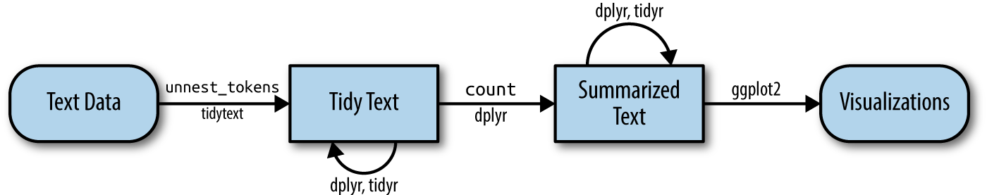
Today, we will explore the tidytext workflow for preprocessing text data. We will focus on the initial steps, as shown in Fig. 1.
Our goals for today are:
Text Data: The example data set we use coming from the State of the Union (SOTU) corpus, which provides a snapshot of the policy priorities of the US executive branch throughout its over 200-year history.
Tidy Text: We will learn how to use the
unnest_tokens()function from thetidytextpackage to tokenize the text data into individual words. We will also discuss the decisions to make when creating a text representation, such as converting text to lowercase, removing stopwords, and lemmatizing or stemming words.Summarized Text: We will use the
count()function fromdplyrto calculate word frequencies and filter the words by frequency.Visualizations: We will create a basic word cloud using the processed text data.
Let’s first install and load the packages.
2 Read in raw data
Two data sets are stored in the sotu package. The dataset sotu_text is a character vector with one address in each element. The dataset sotu_meta provides the context information for each address, such as the president who gave the speech and the year the address was given. Speeches are ordered temporally in sotu_text and can be matched to the rows of sotu_meta.
sotu_meta<-sotu_meta

sotu_text<-sotu_text
Based on the description, we can append these two datasets. In practice, particularly when dealing with a huge amount of text data, it’s often more efficient to preprocess the text data first without linking it to the contextual metadata. This is because the contextual metadata can substantially increase the volume of data and slow down the processing.
sotu <- cbind(sotu_meta, sotu_text) %>%
  rename(doc_id=X) # document unique identification number
Alternatively, you can read-in the data from the shared folder I provided last class. (Hint: use readr)
Notice that this zip file does not include the most recent speeches.
Let’s take a look at the data.
glimpse(sotu)Rows: 240
Columns: 7
$ doc_id <int> 1, 2, 3, 4, 5, 6, 7, 8, 9, 10, 11, 12, 13, 14, 15, 16, 17…
$ president <chr> "George Washington", "George Washington", "George Washing…
$ year <int> 1790, 1790, 1791, 1792, 1793, 1794, 1795, 1796, 1797, 179…
$ years_active <chr> "1789-1793", "1789-1793", "1789-1793", "1789-1793", "1793…
$ party <chr> "Nonpartisan", "Nonpartisan", "Nonpartisan", "Nonpartisan…
$ sotu_type <chr> "speech", "speech", "speech", "speech", "speech", "speech…
$ sotu_text <chr> "Fellow-Citizens of the Senate and House of Representativ…How many speeches each president gave?
sotu %>% group_by(president) %>%
  count(sort=T)  %>%
  rename(num_speeches=n) %>%
  ungroup()
# A tibble: 42 × 2
president num_speeches
<chr> <int>
1 Franklin D. Roosevelt 13
2 Dwight D. Eisenhower 10
3 Andrew Jackson 8
4 Barack Obama 8
5 George W. Bush 8
6 George Washington 8
7 Grover Cleveland 8
8 Harry S Truman 8
9 James Madison 8
10 James Monroe 8
# ℹ 32 more rowssotu %>% group_by(president) %>%
count() %>%
arrange(desc(n)) %>%
rename(num_speeches=n) %>%
ungroup()# A tibble: 42 × 2
president num_speeches
<chr> <int>
1 Franklin D. Roosevelt 13
2 Dwight D. Eisenhower 10
3 Andrew Jackson 8
4 Barack Obama 8
5 George W. Bush 8
6 George Washington 8
7 Grover Cleveland 8
8 Harry S Truman 8
9 James Madison 8
10 James Monroe 8
# ℹ 32 more rowsIf you recall, the above codes is equivalent to using:
 sotu_meta %>%
  group_by(president) %>%
  summarise(num_speeches = n()) %>%
  arrange(desc(num_speeches))
# A tibble: 42 × 2
president num_speeches
<chr> <int>
1 Franklin D. Roosevelt 13
2 Dwight D. Eisenhower 10
3 Andrew Jackson 8
4 Barack Obama 8
5 George W. Bush 8
6 George Washington 8
7 Grover Cleveland 8
8 Harry S Truman 8
9 James Madison 8
10 James Monroe 8
# ℹ 32 more rowsThe output shows a tibble with two columns: president (the name of each president) and num_speeches (the count of speeches given by each president). You can see that the tibble is sorted by the number of speeches for each president from the highest to the lowest.
3 Tokenization
The process of converting text strings into separate words is called tokenization. In tidy text, tokenization is done by unnest_tokens(), restructuring the data frame into a one-token-per-row and long data format.
token_sotu<-sotu %>%
  unnest_tokens(token, #output column
                sotu_text, #input column
                token="words", #unit for tokenizing (default is "words")
                to_lower=T, # convert tokens to lowercase
                drop=F # Do not drop the original input column
)
The resulting token_sotu data frame will have one token (word) per row, with the tokens stored in the token column.
View(token_sotu)Tokenizing English words are relatively simple since distinct words in English are separated using white space. However, in some languages, such as Chinese, Japaneses, and Lao, words are not separated by white spaces.
In these cases, you need to find the corresponding tokenizers or word segmentation models. If you are working on Chinease texts, the package jiebaR (and “jieba” in Python) will be helpful.
4 Pre-processing
After tokenization, we move on to cleaning the unstructured text data to prepare it for analysis. This preprocessing task is a case-by-case decision, and several typical steps are involved, including:
Converting to lowercase
Removing stop words
Removing punctuation
Creating equivalence classes (i.e., stemming/lemmatization)
Filtering by frequency
In the previous tokenization step, each word was converted to lowercase, and all instances of periods, commas, etc., were removed.
4.1 Remove stop words
Stop words are a set of commonly used words in a language, which are less useful for an analysis. In English, stop words are “a,” “the,” “of,” “to,” etc.
data(stop_words)

head(stop_words)
# A tibble: 6 × 2
word lexicon
<chr> <chr>
1 a SMART
2 a's SMART
3 able SMART
4 about SMART
5 above SMART
6 according SMART Like wrangling regular tidy data, we use the functions stop_words and anti_join to exclude the stop words.
token_sotu.clean0<-token_sotu%>%
  anti_join(stop_words,
            by=c("token"="word"))

head(token_sotu.clean0$token,10)
[1] "fellow" "citizens" "senate" "house"
[5] "representatives" "embrace" "satisfaction" "opportunity"
[9] "congratulating" "favorable" Let’s see how much complexity is reduced only by excluding stop words!
message("Reduced row percentage: ",
  round((nrow(token_sotu)-nrow(token_sotu.clean0))/nrow(token_sotu)*100, 2), "%")
Reduced row percentage: 60.37%4.1.1 Tip 1
You can create your own stop words list based on your project needs.
4.1.2 Tip 2
In Chinese, stop words are like “之,” “也,” “了,” “以,” “但,” etc. You can find three commonly used stop words dictionaries here.
Activity 1
Can you think about an alternative way to filter out the stop words from the texts?
token_sotu %>%
slice_head(n=30) %>% # using the first 30 rows as an example
filter(!token %in% stop_words$word) # do not keep a "token" if the "token" is in stop_words' "word"" list.
4.2 Create equivalence classes
You might have noticed that many words carry the same information, such as “governments,” “government’s,” and “government.” It might be effective to map them all to a common form, such as “government.”
This process is called text normalization, which helps to improve the accuracy of many language models. Two methods, stemming and lemmatization, are commonly employed for text normalization.
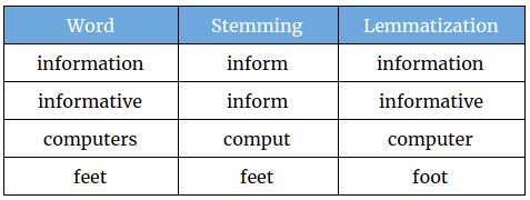
Stemming often involves chopping off the last few characters of a word following simple rules, such as removing “s,” “ed,” and “ty.” There are many stemming algorithms available, each with different rules, such as the Porter Stemmer and the Snowball Stemmer.
Lemmatization, on the other hand, is the process of mapping words to their lemma, which is the canonical form of a word as defined in a dictionary. In most cases, lemmatization tends to be more accurate than stemming. However, as mentioned earlier, the choice between stemming and lemmatization depends on your specific task. See the differences in Fig. 3.
4.2.1 Stemming
token_sotu.clean0.stem<-token_sotu.clean0 %>%
  mutate(stem=stem_words(token, language = "porter"))

token_sotu.clean0.stem %>% select(stem, token) %>%
  head(10)
stem token
1 fellow fellow
2 citizen citizens
3 senat senate
4 hous house
5 repres representatives
6 embrac embrace
7 satisfact satisfaction
8 opportun opportunity
9 congratul congratulating
10 favor favorable4.2.2 Lemmatization
token_sotu.clean0.lemma<-token_sotu.clean0 %>%
  mutate(lemma=lemmatize_words(token))

token_sotu.clean0.lemma %>% select(lemma, token) %>%
  head(10)
lemma token
1 fellow fellow
2 citizen citizens
3 senate senate
4 house house
5 representative representatives
6 embrace embrace
7 satisfaction satisfaction
8 opportunity opportunity
9 congratulate congratulating
10 favorable favorableAs you can see, lemmatization is a better choice for our case. In the following steps, we will use the lemmatized tokens.
4.3 Filter by frequency
We normally remove words that are very rare since they are less likely to provide useful information. Sometimes, we also consider removing words that are very common, depending on the task and model. Removing such words will also save substantial computational power.
Let’s see the frequency list of lemmas, which are our tokens.
token_sotu.count <-token_sotu.clean0.lemma %>%
group_by(lemma) %>%
  count(sort=T)
View(token_sotu.count)
The frequency distribution of lemmas is highly skewed. As you can tell from the median, at least half of the lemmas only occurred twice in the corpus. Also, 75% of lemmas occurred only 11 times. The maximum frequency is 8549! This means one word appears extremely commonly.
summary(token_sotu.count) lemma n
Length:22285 Min. : 1.00
Class :character 1st Qu.: 1.00
Mode :character Median : 2.00
Mean : 35.35
3rd Qu.: 11.00
Max. :8549.00 You can also see the skewness in the following histogram.
ggplot(token_sotu.count,
       aes(x=n)) +
  geom_histogram()
`stat_bin()` using `bins = 30`. Pick better value with `binwidth`.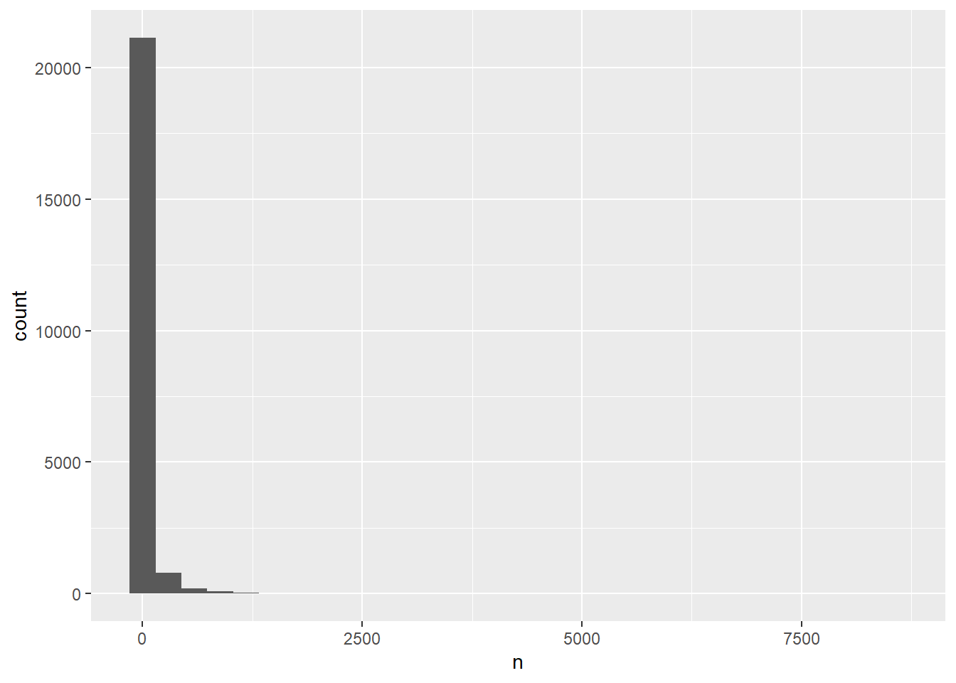
Based on the frequency distribution, we trim the lemmas by excluding the very rare and very common words. The decision on the threshold is arbitrary and depends on the specific task and model. However, some prior examinations (e.g., checking the frequency distribution) are always desirable.
token_sotu.clean1<-token_sotu.clean0.lemma %>%
  group_by(lemma) %>%
  filter(n()>= 5& n()<=4000)
Now, the rows of tokens (which are now lemmas) are further reduced by 6.4%
message("Reduced row percentage: ",
  round((nrow(token_sotu.clean0)-nrow(token_sotu.clean1))/nrow(token_sotu.clean0)*100, 2), "%")
Reduced row percentage: 6.39%5 Word frequencies and word clouds
Now, we can make a wordcloud using ggplot with the geom_text_wordcloud function from the ggwordcloud package.
5.1 Word frequencies
First, we calculate the word frequencies to be used for aesthetics.
word.freq<-token_sotu.clean1 %>%
  group_by(lemma)  %>%
  summarize(termfreq=n(), # The total frequency of each lemma in the corpus
            docfreq=length(unique(doc_id)), #  The number of unique documents (speeches) in which each lemma has occurred,
            relfreq=docfreq/nrow(token_sotu.clean1) # The relative frequency of each lemma
            )  %>%
  arrange(-docfreq) # arrange the rows in descending order of docfreq

word.freq
# A tibble: 8,222 × 4
lemma termfreq docfreq relfreq
<chr> <int> <int> <dbl>
1 nation 3945 239 0.000324
2 time 3672 239 0.000324
3 power 3040 234 0.000317
4 war 3139 233 0.000316
5 national 2488 232 0.000315
6 provide 1987 232 0.000315
7 law 3777 231 0.000313
8 continue 2074 230 0.000312
9 force 1904 230 0.000312
10 peace 2030 230 0.000312
# ℹ 8,212 more rowsThe word.freq data frame shows the calculated frequencies for each lemma, including the term frequency (termfreq), document frequency (docfreq), and relative frequency (relfreq).
The relative frequency of each lemma can be interpreted as the proportion or percentage of tokens in the entire corpus that belong to a particular lemma. For example, a lemma has a 0.05 relative frequency means that 5% of the tokens in the entire corpus belong to that particular lemma. In this case, the higher the relative frequency of a lemma, the more important or prevalent it is considered to be in the context of the entire corpus.
5.2 Word clouds
Now, let’s create the word cloud using ggplot2 and geom_text_wordcloud. Do you recall the grammar of graphics in ggplot2?
word.freq %>%
  slice_max(termfreq, n=150)  %>% # Select the top 150 lemmas based on their term frequency
  ggplot(aes(label=lemma, # The lemma to be displayed as text in the word cloud
             size=termfreq, # The size of each word, proportional to its term frequency
             color=relfreq) # The color of each word, representing its relative frequency
         )+
  geom_text_wordcloud()+ # Geometry function for
  theme_minimal() # set a minimal theme for the plot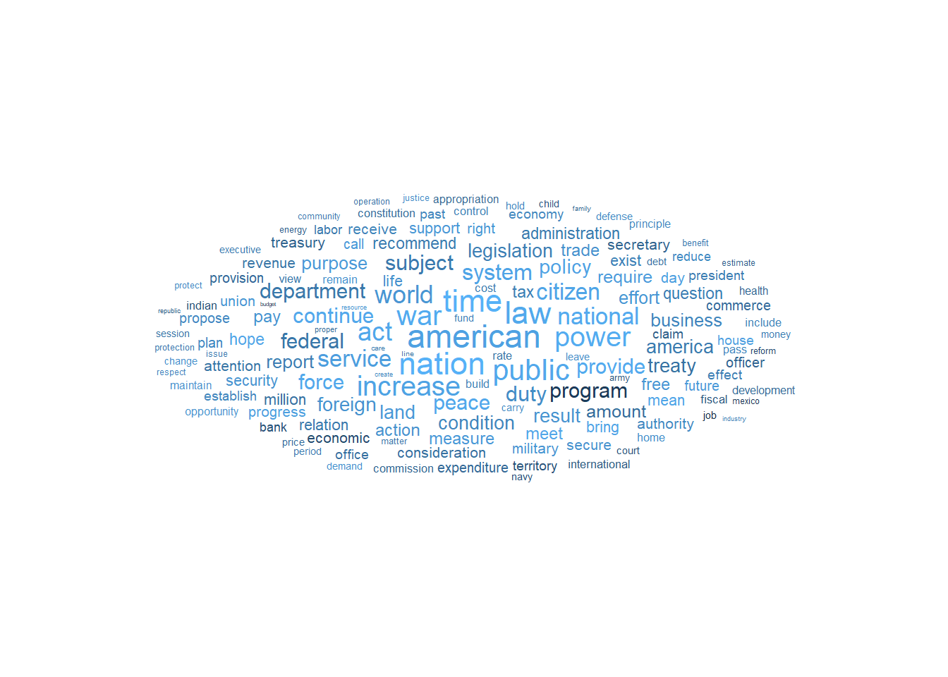
Finally, we have the word cloud that visualizes the top 150 most frequently appearing lemmas, allowing us to quickly identify the most prominent and widely used words in SOTU!
5.2.1 Activity 2
Can you make comparisons of two presidents’ speeches using word clouds?