#install.packages(c("quanteda", "quanteda.textstats", "quanteda.textplots"))


library(quanteda)
library(quanteda.textstats)
library(quanteda.textplots)

library(sotu)
library(tidyverse)Bag of Words
Session 3b
1 Bag-of-words (BOW)
Bag of words and word embeddings are two main representations of the corpus and documents we collected. The core idea of Bag of words is simple: we will present each document by counting how many times each word appears in it. (Grimmer et al., 2022, p48)
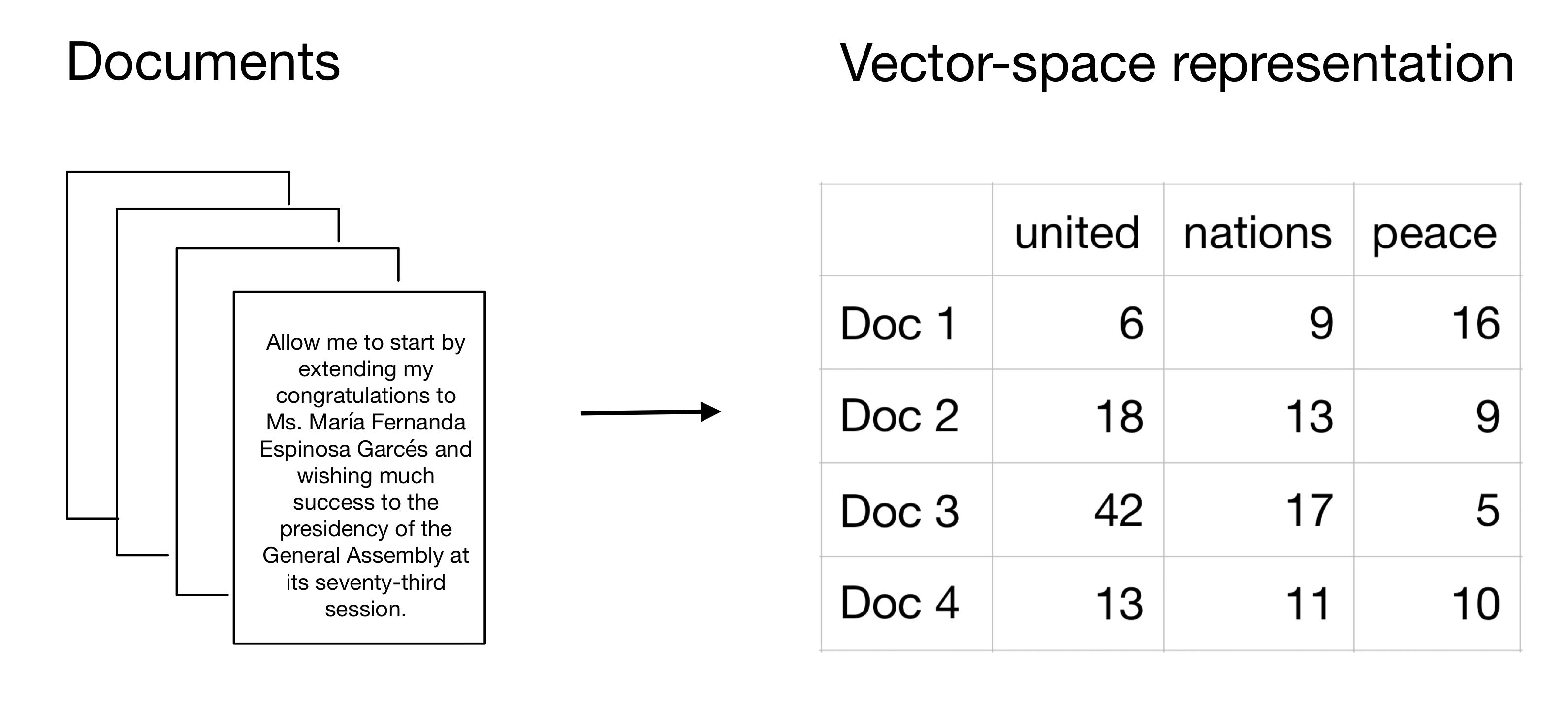
With this representation, we will compute a document-feature matrix (DFM), also known as a document-term matrix (DTM).
In a DFM, each row corresponds to a document in the corpus, and each column corresponds to a unique term or feature in the vocabulary. See Fig.1, showing a DFM in where the feature is the count of terms (i.e., words) appeared in each document.
2 Conducting text analysis in quanteda
Previously, we worked on the tidy way to tokenize and preprocessing text data, using tidytext. Another R package, called quanteda, provides a comprehensive set of tools for quantitative text analysis and offers flexibility in working with both non-tidy and tidy data structures.
In this class, we will explore how to use quanteda for BOW and continue to use the State of the Union (SOTU) corpus from the sotu package as our example dataset.
2.1 Load packages and data
quanteda is powerful to be used with its extensions, see quanteda family here.
Load the SOTU dataset.
sotu_text <-sotu_text
sotu_meta <-sotu_meta
2.2 Constructing DFM
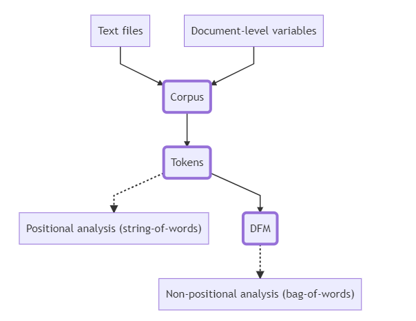
In quanteda, we need to build three basic types of objects: corpus, tokens, and dfm. See Fig.2 presented below.
Let’s work through these three objects together and start with creating a corpus object.
# Create a corpus
sotu_corpus <- corpus(sotu_text,
                      docvars=sotu_meta)
The metadata associated with each document is specified using docvars.
head(docvars(sotu_corpus)) X president year years_active party sotu_type
1 1 George Washington 1790 1789-1793 Nonpartisan speech
2 2 George Washington 1790 1789-1793 Nonpartisan speech
3 3 George Washington 1791 1789-1793 Nonpartisan speech
4 4 George Washington 1792 1789-1793 Nonpartisan speech
5 5 George Washington 1793 1793-1797 Nonpartisan speech
6 6 George Washington 1794 1793-1797 Nonpartisan speechSecond, we build tokens with preprocessing, which is stored in a list of vectors
sotu_toks_clean <- sotu_corpus %>%
  tokens(remove_punct = TRUE) %>%
  tokens_tolower() %>%
  tokens_remove(stopwords("en"))
Finally, we construct a document-feature matrix (DFM) using the dfm() function from quanteda.
# Create a DFM
sotu_dfm <- dfm(sotu_toks_clean)
The dfm object now contains the document-feature matrix, where each row represents a document and each column represents a term.
print(sotu_dfm)Document-feature matrix of: 240 documents, 32,816 features (94.82% sparse) and 6 docvars.
features
docs fellow-citizens senate house representatives embrace great satisfaction
text1 1 2 3 3 1 4 2
text2 1 2 3 3 0 4 1
text3 1 3 3 3 0 0 3
text4 1 2 3 3 0 0 3
text5 1 2 3 3 0 0 0
text6 1 2 4 3 0 1 0
features
docs opportunity now presents
text1 1 1 1
text2 0 2 0
text3 1 0 0
text4 0 2 0
text5 1 2 0
text6 1 3 0
[ reached max_ndoc ... 234 more documents, reached max_nfeat ... 32,806 more features ]You can get the number of documents and features (i.e., tokens) using ndoc() and nfeat().
ndoc(sotu_dfm)[1] 240nfeat(sotu_dfm)[1] 328163 Dictionary-Based sentiment analysis
In quanteda, we can perform dictionary-based sentiment analysis using the dfm_lookup() function. Showing an example, we use a predefined sentiment dictionary of “LSD 2015 dictionary”. In practice, you should search for the lexicon that best suit for your work needs.
data("data_dictionary_LSD2015")sotu_sentiment_scores <- dfm_lookup(sotu_dfm,
dictionary = data_dictionary_LSD2015)
# Display the sentiment scores
head(sotu_sentiment_scores)Document-feature matrix of: 6 documents, 4 features (50.00% sparse) and 6 docvars.
features
docs negative positive neg_positive neg_negative
text1 16 127 0 0
text2 37 107 0 0
text3 62 185 0 0
text4 68 130 0 0
text5 76 143 0 0
text6 141 204 0 0The sotu_sentiment_scores object contains the sentiment scores for each document based on the sentiment dictionary.
4 Generate n-grams
As we have seen the Google Book ngram Viewer showing the trends of words and phrases, ngrams are sequences of n adjacent words. When n=1, it is called unigrams, which is equivalent to the individual word we tokenized above. When n=2 and n=3, the ngrams are bigrams and trigrams correspondingly. When n>3, we referred to four or five grams and so on.Ver
Let’s tokenize the sotu text by 2-grams, i.e., bigram, to take a closer look of ngrams.
suto_toks_bigram <- sotu_corpus %>%
  tokens(remove_punct = TRUE) %>%
  tokens_tolower() %>%
  tokens_remove(stopwords("en")) %>%
tokens_ngrams(n = 2)head(suto_toks_bigram[[1]], 30) [1] "fellow-citizens_senate" "senate_house"
[3] "house_representatives" "representatives_embrace"
[5] "embrace_great" "great_satisfaction"
[7] "satisfaction_opportunity" "opportunity_now"
[9] "now_presents" "presents_congratulating"
[11] "congratulating_present" "present_favorable"
[13] "favorable_prospects" "prospects_public"
[15] "public_affairs" "affairs_recent"
[17] "recent_accession" "accession_important"
[19] "important_state" "state_north"
[21] "north_carolina" "carolina_constitution"
[23] "constitution_united" "united_states"
[25] "states_official" "official_information"
[27] "information_received" "received_rising"
[29] "rising_credit" "credit_respectability" You can see that one bigram moves one word forward to generate the next bigram.
With this characteristic, unlike individual words, ngram provides the sequence or order of words and it is often used for predicting the occurrence probability of a word based on the occurrence of previous words.
In our case, we also want to keep the commonly used phrases or terms, such as “federal government”, that bridged by multiple words.
suto_toks_bigram_select <- tokens_select(suto_toks_bigram, pattern = phrase("*_government"))


head(suto_toks_bigram_select, 15)
Tokens consisting of 15 documents and 6 docvars.
text1 :
[1] "toward_government" "measures_government" "end_government"
[4] "equal_government"
text2 :
[1] "present_government" "sensible_government" "established_government"
text3 :
[1] "confidence_government" "acts_government"
[3] "seat_government" "new_government"
[5] "convenience_government" "arrangements_government"
[7] "proceedings_government"
text4 :
[1] "departments_government" "reserved_government"
[3] "constitution_government"
text5 :
[1] "republican_government" "firm_government" "welfare_government"
text6 :
[1] "character_government" "irresolution_government"
[3] "seat_government" "conduct_government"
[5] "friends_government" "tendered_government"
[7] "good_government" "seat_government"
[9] "emergencies_government" "principles_government"
[11] "republican_government" "whole_government"
[ ... and 2 more ]
[ reached max_ndoc ... 9 more documents ]
Tip
For advanced analyses on ngrams, I recommend to convert the quanteda dfm object into the tidy ones. See the last section on converting between tidy and non-tidy objects. I strongly encourage you to explore this conversion system to accelerate your text-as-data project.
5 Trim the sparsity of a DFM
We can trim the sparsity of the DFM by removing terms that appear in less than a specified number of documents using the dfm_trim() function.
# Trim the sparsity of the DFM
sotu_dfm_trimmed <- dfm_trim(sotu_dfm,
                             min_docfreq = 2) # remove the terms appeared in less than 2 documents
The sotu_dfm_trimmed object now contains the trimmed DFM, where terms appearing in less than 2 documents have been removed.
summary(sotu_dfm_trimmed) Length Class Mode
4399200 dfm S4 There are many other ways of trimming a dfm for sparsity reason, check out the general rules we suggested in the class and the options provided in dfm_trim().
?dfm_trimstarting httpd help server ... done6 Comparing documents
In quanteda, we use textstat_simil() and textstat_dist()to calculate the closeness of documents
6.1 Cosine similarity
sotu_cosine <- textstat_simil(sotu_dfm,
                              method = "cosine",
                              margin = "documents" # here we compare the documents (i.e., the speeches); if you want to compare the tokens, specify margin = "feature"
                              )
The output will be a similarity matrix, which is a square matrix that contains pairwise similarity scores between documents. - Each cell (i, j) represents the similarity between document i and document j - Similarity matrices are symmetric, with the diagonal elements representing self-similarity (which is 1)
str(sotu_cosine)Formal class 'textstat_simil_symm' [package "quanteda.textstats"] with 8 slots
..@ method : chr "cosine"
..@ margin : chr "documents"
..@ type : chr "textstat_simil"
..@ Dim : int [1:2] 240 240
..@ Dimnames:List of 2
.. ..$ : chr [1:240] "text1" "text2" "text3" "text4" ...
.. ..$ : chr [1:240] "text1" "text2" "text3" "text4" ...
..@ uplo : chr "U"
..@ x : num [1:28920] 1 0.478 1 0.529 0.474 ...
..@ factors : list()Let’s take a quick look of the first speech’s similarity with the following 20 ones. Do you recall how to select matrix element in our very first R session?
matrix.sotu_cosine<-as.matrix(sotu_cosine)

matrix.sotu_cosine[1, # selecting the 1st row
                       1:20] # selecting 1st column to the 20th
text1 text2 text3 text4 text5 text6 text7 text8
1.0000000 0.4781219 0.5293360 0.4634483 0.4283547 0.4136844 0.4823802 0.4917780
text9 text10 text11 text12 text13 text14 text15 text16
0.4078687 0.4475699 0.4065614 0.4487946 0.4297602 0.3543613 0.3917148 0.3843641
text17 text18 text19 text20
0.3752920 0.4526491 0.3840181 0.4115510 The mean of the cosine similarity of the first documents is about 0.35
mean(matrix.sotu_cosine[1,2:ncol(matrix.sotu_cosine)])[1] 0.3535386Let’s see 10 documents that are most similar to the first document, which are, unsurprisingly, all larger than the mean cosine similarity.
text1_10_cosine<-head(sort(sotu_cosine[1,],
                      dec=T), 11)

text1_10_cosine
text1 text3 text42 text44 text41 text62 text50 text48
1.0000000 0.5293360 0.5244950 0.5211707 0.5203932 0.5061035 0.4966398 0.4930177
text8 text64 text7
0.4917780 0.4882689 0.4823802 You can see from the Environment that text1_10_cosine is a named vector (i.e., a numeric vector with names). We can wrangle it and merge with sotu_meta to know the meta data providing contextual information, such as who are the presidents, of these similar documents.
text1_10_cosine.df<-text1_10_cosine %>%
  as.data.frame() %>% # converting the named vector to a data frame
  rownames_to_column() %>%  # setting the text* row to the first column
  set_names(c("T10_doc_id", "cosine_tfidf")) %>% # assigning column names
  mutate(T10_doc_id=str_remove(T10_doc_id, "text"), # removing the common prefix of the first column to be merged with the sotu_meta data
         T10_doc_id=as.numeric(T10_doc_id)) %>% # making sure the key variables for the following join task are in the same type.
  inner_join(sotu_meta %>% cbind(sotu_text), # you can use pip to link the meta and text data within a function!
             by=c("T10_doc_id"="X"))
Let’s take a glimpse of the merged data. Who are the orators and when were the speeches given?
glimpse(text1_10_cosine.df)Rows: 11
Columns: 8
$ T10_doc_id <dbl> 1, 3, 42, 44, 41, 62, 50, 48, 8, 64, 7
$ cosine_tfidf <dbl> 1.0000000, 0.5293360, 0.5244950, 0.5211707, 0.5203932, 0.…
$ president <chr> "George Washington", "George Washington", "Andrew Jackson…
$ year <int> 1790, 1791, 1830, 1832, 1829, 1850, 1838, 1836, 1796, 185…
$ years_active <chr> "1789-1793", "1789-1793", "1829-1833", "1829-1833", "1829…
$ party <chr> "Nonpartisan", "Nonpartisan", "Democratic", "Democratic",…
$ sotu_type <chr> "speech", "speech", "written", "written", "written", "wri…
$ sotu_text <chr> "Fellow-Citizens of the Senate and House of Representativ…It seems like the speeches given by Preseident Andrew Jackson are the most similar to the first speech given by President George Washington.
text1_10_cosine.df$president [1] "George Washington" "George Washington" "Andrew Jackson"
[4] "Andrew Jackson" "Andrew Jackson" "Millard Fillmore"
[7] "Martin Van Buren" "Andrew Jackson" "George Washington"
[10] "Millard Fillmore" "George Washington"text1_10_cosine.df$party [1] "Nonpartisan" "Nonpartisan" "Democratic" "Democratic" "Democratic"
[6] "Whig" "Democratic" "Democratic" "Nonpartisan" "Whig"
[11] "Nonpartisan"6.2 Jaccard similarity
Similarly, we compute the jaccard similarity using textstat_simil() with speycifying the method argument to be "jaccard".
sotu_jaccard <- textstat_simil(sotu_dfm,
                              method = "jaccard",
                              margin = "documents")
Again, we check the ten documents that are most similar to the first document in terms of jaccard similarity.
text1_10_jaccard<-head(sort(sotu_jaccard[1,],
                      dec=T), 11)

text1_10_jaccard
text1 text3 text2 text4 text7 text15 text5 text22
1.0000000 0.2044199 0.1904762 0.1852273 0.1677419 0.1594509 0.1581243 0.1560000
text27 text10 text8
0.1545936 0.1537646 0.1519337 Let’s see who given these most similar documents.
text1_10_jaccard.df<-text1_10_jaccard %>%
  as.data.frame() %>%
  rownames_to_column() %>%
  set_names(c("T10_doc_id", "jaccard")) %>%
  mutate(T10_doc_id=str_remove(T10_doc_id, "text"),
         T10_doc_id=as.numeric(T10_doc_id)) %>%
  inner_join(sotu_meta %>% cbind(sotu_text),
             by=c("T10_doc_id"="X"))

glimpse(text1_10_jaccard.df)
Rows: 11
Columns: 8
$ T10_doc_id <dbl> 1, 3, 2, 4, 7, 15, 5, 22, 27, 10, 8
$ jaccard <dbl> 1.0000000, 0.2044199, 0.1904762, 0.1852273, 0.1677419, 0.…
$ president <chr> "George Washington", "George Washington", "George Washing…
$ year <int> 1790, 1791, 1790, 1792, 1795, 1803, 1793, 1810, 1815, 179…
$ years_active <chr> "1789-1793", "1789-1793", "1789-1793", "1789-1793", "1793…
$ party <chr> "Nonpartisan", "Nonpartisan", "Nonpartisan", "Nonpartisan…
$ sotu_type <chr> "speech", "speech", "speech", "speech", "speech", "writte…
$ sotu_text <chr> "Fellow-Citizens of the Senate and House of Representativ…
Activity
Using the jaccard similarity measures, can you find who are the orators have the most similar speeches with the first speech given by President George Washington?
6.3 Euclidean distance
We now switch to the distance measure using textstat_dist(). Again, we only need to specify the distance measure in method=
sotu_euclidean <- textstat_dist(sotu_dfm,
                              method = "euclidean",
                              margin = "documents")
The 10 most “distanced” documents from the first documents:
text1_10_euclidean<-head(sort(sotu_euclidean[1,],
                      dec=F), # notice that we want to find the smallest distances to detect the most similar documents!
                      11)

text1_10_euclidean
text1 text2 text12 text11 text169 text7 text21 text4
0.00000 32.09361 35.25621 37.77565 38.56164 38.76854 40.68169 42.00000
text10 text16 text3
46.07602 46.17359 46.45428 Who are the oraters and their parties?
text1_10_euclidean.df<-text1_10_euclidean %>%
  as.data.frame() %>%
  rownames_to_column() %>%
  set_names(c("T10_doc_id", "euclidean")) %>%
  mutate(T10_doc_id=str_remove(T10_doc_id, "text"),
         T10_doc_id=as.numeric(T10_doc_id)) %>%
  inner_join(sotu_meta %>% cbind(sotu_text),
             by=c("T10_doc_id"="X"))

glimpse(text1_10_euclidean.df)
Rows: 11
Columns: 8
$ T10_doc_id <dbl> 1, 2, 12, 11, 169, 7, 21, 4, 10, 16, 3
$ euclidean <dbl> 0.00000, 32.09361, 35.25621, 37.77565, 38.56164, 38.76854…
$ president <chr> "George Washington", "George Washington", "John Adams", "…
$ year <int> 1790, 1790, 1800, 1799, 1956, 1795, 1809, 1792, 1798, 180…
$ years_active <chr> "1789-1793", "1789-1793", "1797-1801", "1797-1801", "1953…
$ party <chr> "Nonpartisan", "Nonpartisan", "Federalist", "Federalist",…
$ sotu_type <chr> "speech", "speech", "speech", "speech", "speech", "speech…
$ sotu_text <chr> "Fellow-Citizens of the Senate and House of Representativ…6.4 TF-IDF
The above closeness measures were calculated based on the unweighted dfm and vector space model.
The following shows how to weight the words using TF-IDF. To do so, we use function dfm_tfidf().
sotu_dfm_tfidf <- dfm_tfidf(sotu_dfm)With the TF-IDF weighting applied, let’s calculate the cosine similarity again.
sotu_cosine_tfidf <- textstat_simil(sotu_dfm_tfidf,
                                    method = "cosine",
                                    margin = "documents")
The most similar ten documents with the first document after the weighting are then:
text1_10_cosine_tfidf<-head(sort(sotu_cosine_tfidf[1,],
                      dec=T), 11)

text1_10_cosine_tfidf
text1 text3 text2 text42 text4 text36 text37 text41
1.0000000 0.1784764 0.1417079 0.1384592 0.1333127 0.1310056 0.1156438 0.1106553
text7 text48 text29
0.1091577 0.1076958 0.1020808 text1_10_cosine_tfidf.df<-text1_10_cosine_tfidf %>%
as.data.frame() %>%
rownames_to_column() %>%
set_names(c("T10_doc_id", "cosine_tfidf")) %>%
mutate(T10_doc_id=str_remove(T10_doc_id, "text"),
T10_doc_id=as.numeric(T10_doc_id)) %>%
inner_join(sotu_meta %>% cbind(sotu_text),
by=c("T10_doc_id"="X"))
glimpse(text1_10_cosine_tfidf.df)Rows: 11
Columns: 8
$ T10_doc_id <dbl> 1, 3, 2, 42, 4, 36, 37, 41, 7, 48, 29
$ cosine_tfidf <dbl> 1.0000000, 0.1784764, 0.1417079, 0.1384592, 0.1333127, 0.…
$ president <chr> "George Washington", "George Washington", "George Washing…
$ year <int> 1790, 1791, 1790, 1830, 1792, 1824, 1825, 1829, 1795, 183…
$ years_active <chr> "1789-1793", "1789-1793", "1789-1793", "1829-1833", "1789…
$ party <chr> "Nonpartisan", "Nonpartisan", "Nonpartisan", "Democratic"…
$ sotu_type <chr> "speech", "speech", "speech", "written", "speech", "writt…
$ sotu_text <chr> "Fellow-Citizens of the Senate and House of Representativ…Can we see any changes from the original cosine similarity matrix, and the other similarity matrices?
cosine_tfidf_T10orators <-text1_10_cosine_tfidf.df$president

cosine_T10orators <-text1_10_cosine.df$president
jaccard_T10orators <-text1_10_jaccard.df$president
euclidean_T10orators <-text1_10_euclidean.df$president

comp.df<-data.frame(cosine_T10orators, cosine_tfidf_T10orators, jaccard_T10orators,euclidean_T10orators)
comp.df
cosine_T10orators cosine_tfidf_T10orators jaccard_T10orators
1 George Washington George Washington George Washington
2 George Washington George Washington George Washington
3 Andrew Jackson George Washington George Washington
4 Andrew Jackson Andrew Jackson George Washington
5 Andrew Jackson George Washington George Washington
6 Millard Fillmore James Monroe Thomas Jefferson
7 Martin Van Buren John Quincy Adams George Washington
8 Andrew Jackson Andrew Jackson James Madison
9 George Washington George Washington James Madison
10 Millard Fillmore Andrew Jackson John Adams
11 George Washington James Monroe George Washington
euclidean_T10orators
1 George Washington
2 George Washington
3 John Adams
4 John Adams
5 Dwight D. Eisenhower
6 George Washington
7 James Madison
8 George Washington
9 John Adams
10 Thomas Jefferson
11 George Washington6.5 Keyness test
We can also conduct a keyness test to compare the frequency of words between two parties using the textstat_keyness() function.
# Perform keyness test
sotu_keyness <- textstat_keyness(sotu_dfm,
                                 target = sotu_dfm$party=="Democratic")


# Display the keyness results}
head(sotu_keyness, n = 20)
feature chi2 p n_target n_reference
1 million 217.19232 0 544 252
2 bank 167.57163 0 308 109
3 program 152.74891 0 691 449
4 soviet 148.14226 0 269 94
5 jobs 143.84605 0 408 206
6 mexico 142.60358 0 543 325
7 energy 133.20192 0 511 307
8 1980 132.09519 0 136 18
9 1947 121.41339 0 97 3
10 nuclear 115.27943 0 260 111
11 1979 111.06405 0 87 2
12 dollars 110.57066 0 359 197
13 1978 108.12186 0 80 0
14 world 102.99443 0 1356 1233
15 businesses 101.42865 0 147 39
16 continue 99.18413 0 638 476
17 u.s 96.51049 0 127 29
18 health 94.98306 0 561 406
19 know 94.79107 0 462 310
20 college 93.98577 0 136 36The keyness object shows the top 20 keywords that are significantly more frequent in the Democratic party compared to the other. A positive keyness value indicates overuse in the target group, while a negative value indicates underuse.
textplot_keyness(sotu_keyness)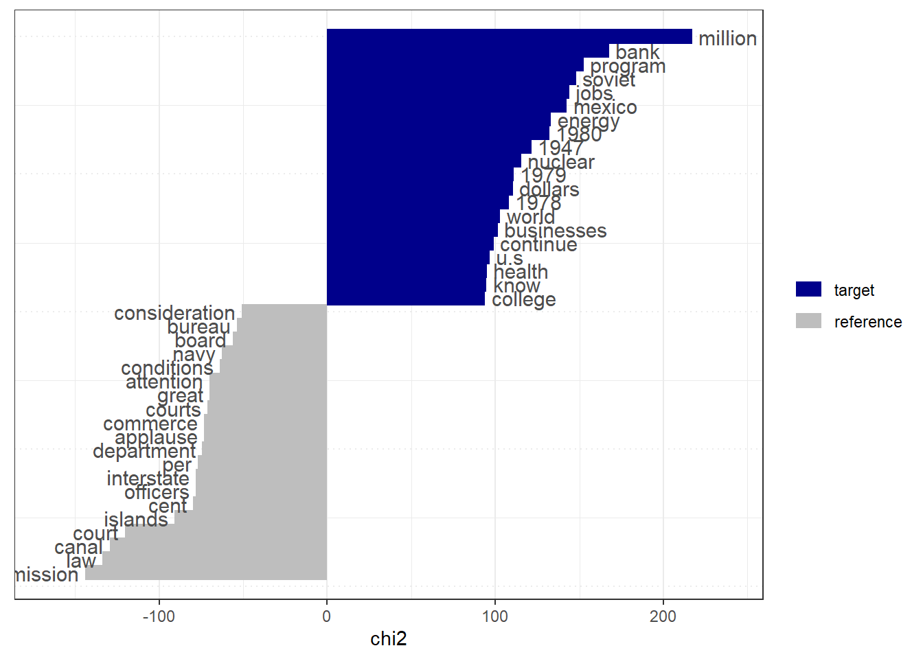
7 Switching between non-tidy and tidy formats
In this tutorial, we used the quanteda package, which works with non-tidy data structures like dfm. If you prefer working with tidy data structures, you can use the convert() function from quanteda to convert a DFM to a tidy format compatible with the tidytext package. This allows you to leverage the tidy data principles and use functions from tidytext for further analysis.
For example:
# Convert DFM to tidy format
tidy_sotu_dfm <- convert(sotu_dfm, to = "data.frame")
The tidy_dfm object now contains the DFM in a tidy format, where each row represents a unique document-term combination.
For more information on switching between non-tidy and tidy formats, you can refer to the quanteda documentation and the chapter 5 from “Text mining with R: A tidy approach” by Julia Silge and David Robinson (https://www.tidytextmining.com/).